Thermometer plots in Excel

In the last post about Thermometer plots in R, I updated with a quick example of something similar in Excel.  John asked how it was done.

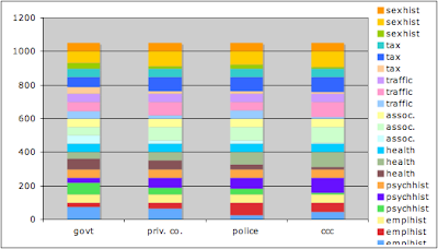
It is a stacked column chart with some dummy series.



For each category, there is one row of data, one row of 100 minus the data, and one row of a gap = 50.

The first version of the chart shows all the series.



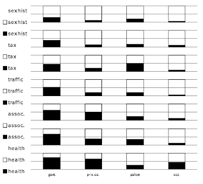
Now we format all the data to be the same - here black lines with black fill.
Format the 100 - data to be the empty part of the thermometer.  In the last post I used gray; here I use black lines with no fill.
Format the gaps as no lines, no fill.
Adjust the grid lines to 50 to match up with the gaps.  Further tidy up.

 
Finally for the legend, we can remove the individual entries for the data and 100-data.  This leaves only the legends for the gaps, which do not have any symbols with them.

Note that when you remove entries from the legend, select the legend, then select the entry, then delete. Make sure you select the whole entry, rather than just the symbol (e.g., the little black square). Otherwise you will delete the whole data series instead of just the legend entry.

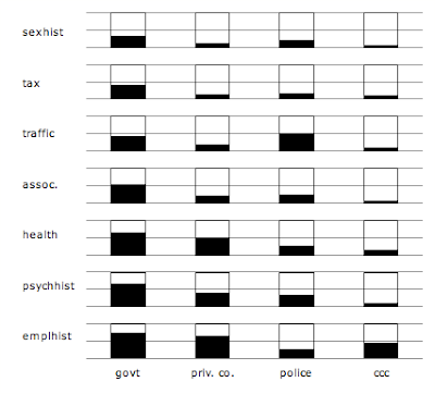
Finally, if we want to look a bit more like the R version, we can eliminate the grid on the whole chart and just put in the 50% markers on each thermometer.  Beyond saying this involves another row of dummy data, I'll leave this as an execise for the reader.